The Foundation of AI Problem Solving
Graph traversal algorithms form the backbone of countless AI applications, yet their importance is often overlooked in favor of more glamorous machine learning techniques.
Graph traversal algorithms form the backbone of countless AI applications, yet their importance is often overlooked in favor of more glamorous machine learning techniques. And so today, I will delve into two cornerstone algorithms that have quietly powered AI systems for decades: Depth-First Search (DFS) and Breadth-First Search (BFS). From neural network architectures to reinforcement learning strategies, these fundamental methods serve as the invisible foundation upon which modern AI systems navigate complex problem spaces. Understanding these traversal algorithms provides both theoretical insights and practical tools essential for creating robust AI solutions.
In the vast landscape of artificial intelligence and computer science, few concepts are as fundamental and widely applicable as graph traversal algorithms. Among these, Depth-First Search (DFS) and Breadth-First Search (BFS) stand as cornerstones that have shaped how we approach problem-solving in AI systems. Understanding these algorithms is not merely an academic exercise; rather, it provides crucial insights into how intelligent systems navigate complex decision spaces and find solutions to challenging problems. I will use Python for all the implementation examples here.
Understanding Graph Theory in AI Context
To fully appreciate the power of DFS and BFS, we must first establish the foundational concept that underlies both algorithms: graph theory. In computer science and AI, a graph represents a collection of nodes (also called vertices) connected by edges. This abstract mathematical structure proves remarkably versatile for modeling real-world problems that AI systems encounter daily.
Consider how an AI navigation system works. Each intersection represents a node, while roads connecting these intersections form edges. Similarly, in game-playing AI like chess engines, each possible board state constitutes a node, with legal moves creating edges between states. This graph-based representation allows AI systems to systematically explore possible solutions, making informed decisions about which paths to pursue.
Moreover, the power of graph representation extends far beyond these simple examples. Social networks, knowledge bases, neural network architectures, and decision trees all utilize graph structures. Consequently, understanding how to traverse these graphs effectively becomes essential for developing robust AI systems.
Depth-First Search: Diving Deep into Solution Spaces
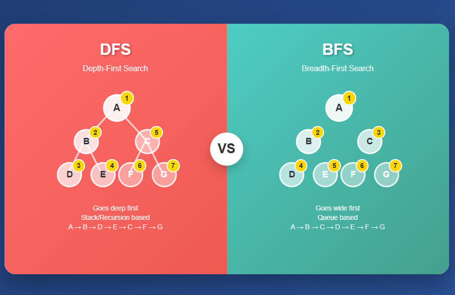
Building upon our understanding of graph theory, let's explore our first traversal algorithm: Depth-First Search. DFS represents one of the most intuitive approaches to graph exploration. As its name suggests, DFS prioritizes depth over breadth, meaning it explores as far as possible along each branch before backtracking to explore alternative paths. This characteristic makes DFS particularly valuable in scenarios where we need to find any solution quickly or when we're working with limited memory resources.
From an implementation perspective, the algorithm operates using a stack data structure, either explicitly implemented or implicitly through recursive function calls. When DFS encounters a node, it immediately explores one of its unvisited neighbors, continuing this process until it reaches a dead end. Only then does it backtrack to the most recent node with unexplored neighbors and continue the search from there.
def depth_first_search(graph, start, target):
    """
    Perform DFS to find a path from start to target node.

    Args:
        graph: Dictionary representing adjacency list
        start: Starting node
        target: Target node to find

    Returns:
        List representing the path from start to target, or None if no path exists
    """
    stack = [(start, [start])]  # (current_node, path_to_current)
    visited = set()

    while stack:
        current_node, path = stack.pop()

        if current_node == target:
            return path

        if current_node not in visited:
            visited.add(current_node)

            # Add neighbors to stack (in reverse order to maintain left-to-right exploration)
            for neighbor in reversed(graph.get(current_node, [])):
                if neighbor not in visited:
                    stack.append((neighbor, path + [neighbor]))

    return None  # No path found

# Example usage
graph = {
    'A': ['B', 'C'],
    'B': ['D', 'E'],
    'C': ['F'],
    'D': [],
    'E': ['F'],
    'F': []
}

result = depth_first_search(graph, 'A', 'F')
print(f"DFS path from A to F: {result}")
While the iterative approach offers excellent control over memory usage, the recursive implementation of DFS often provides cleaner, more readable code, particularly when dealing with tree structures or when the call stack depth is manageable:
def dfs_recursive(graph, current, target, visited=None, path=None):
    """
    Recursive implementation of DFS.

    Args:
        graph: Dictionary representing adjacency list
        current: Current node being explored
        target: Target node to find
        visited: Set of already visited nodes
        path: Current path from start to current node

    Returns:
        List representing the path from start to target, or None if no path exists
    """
    if visited is None:
        visited = set()
    if path is None:
        path = []

    visited.add(current)
    path = path + [current]

    if current == target:
        return path

    for neighbor in graph.get(current, []):
        if neighbor not in visited:
            result = dfs_recursive(graph, neighbor, target, visited, path)
            if result:
                return result

    return None
Breadth-First Search: Exploring Layer by Layer
Having examined DFS's depth-oriented approach, we now turn to its counterpart: Breadth-First Search. In contrast to DFS, BFS explores graphs systematically by examining all nodes at the current depth level before moving to the next level. This methodical exploration pattern makes BFS particularly valuable when we need to find the shortest path between two nodes or when we want to explore solutions in order of their distance from the starting point.
In terms of implementation, BFS utilizes a queue data structure to maintain the order of node exploration. This FIFO (First-In-First-Out) approach ensures that nodes are processed in the order they were discovered, guaranteeing that closer nodes are always explored before more distant ones.
from collections import deque

def breadth_first_search(graph, start, target):
    """
    Perform BFS to find the shortest path from start to target node.

    Args:
        graph: Dictionary representing adjacency list
        start: Starting node
        target: Target node to find

    Returns:
        List representing the shortest path from start to target, or None if no path exists
    """
    queue = deque([(start, [start])])  # (current_node, path_to_current)
    visited = set([start])

    while queue:
        current_node, path = queue.popleft()

        if current_node == target:
            return path

        for neighbor in graph.get(current_node, []):
            if neighbor not in visited:
                visited.add(neighbor)
                queue.append((neighbor, path + [neighbor]))

    return None  # No path found

# Example usage with the same graph
result = breadth_first_search(graph, 'A', 'F')
print(f"BFS path from A to F: {result}")
At this point, it's important to highlight the key distinction between DFS and BFS when we consider their exploration patterns. While DFS might find a solution quickly if it happens to explore the correct branch first, BFS guarantees finding the shortest path in terms of the number of edges traversed. This property makes BFS invaluable in many AI applications where optimality matters.
Comparative Analysis: When to Choose DFS vs BFS
Given these fundamental differences between the two algorithms, the choice between DFS and BFS depends heavily on the specific requirements of your AI application. Each algorithm offers distinct advantages that make it more suitable for certain types of problems.
Memory Considerations and Space Complexity
When evaluating these algorithms, one of the first factors to consider is their memory requirements. From a memory perspective, DFS generally requires less space than BFS. DFS's space complexity is O(h), where h represents the maximum depth of the graph, since it only needs to maintain the current path in memory. In contrast, BFS requires O(w) space, where w represents the maximum width of the graph, as it must store all nodes at the current level in its queue.
As a result, this difference becomes particularly significant when dealing with wide, shallow graphs versus narrow, deep graphs. For instance, when exploring a binary tree with millions of nodes, DFS would require memory proportional to the tree's height (typically log n for balanced trees), while BFS might need to store thousands of nodes simultaneously at each level.
Time Complexity and Solution Quality
Moving beyond memory considerations, we must also examine the temporal and qualitative aspects of these algorithms. Both algorithms share the same time complexity of O(V + E), where V represents the number of vertices and E represents the number of edges. However, their practical performance can vary significantly based on the problem structure and solution location.
Specifically, DFS excels when solutions are likely to be found deep in the search space or when any solution suffices. It can potentially find solutions much faster than BFS if the solution happens to lie along the first path explored. Conversely, BFS guarantees optimal solutions in unweighted graphs, making it essential when solution quality matters more than discovery speed.
def compare_algorithms(graph, start, target):
    """
    Compare DFS and BFS performance on the same graph.

    Args:
        graph: Dictionary representing adjacency list
        start: Starting node
        target: Target node to find

    Returns:
        Dictionary containing results from both algorithms
    """
    import time

    # Measure DFS performance
    start_time = time.time()
    dfs_path = depth_first_search(graph, start, target)
    dfs_time = time.time() - start_time

    # Measure BFS performance
    start_time = time.time()
    bfs_path = breadth_first_search(graph, start, target)
    bfs_time = time.time() - start_time

    return {
        'dfs': {'path': dfs_path, 'length': len(dfs_path) if dfs_path else None, 'time': dfs_time},
        'bfs': {'path': bfs_path, 'length': len(bfs_path) if bfs_path else None, 'time': bfs_time}
    }

# Example comparison
results = compare_algorithms(graph, 'A', 'F')
print("Algorithm Comparison Results:")
print(f"DFS: {results['dfs']}")
print(f"BFS: {results['bfs']}")
Applications in Artificial Intelligence Systems
With our understanding of both algorithms and their comparative advantages established, let's explore how DFS and BFS manifest in real-world AI applications. The practical applications of these algorithms in AI systems are remarkably diverse, spanning from fundamental pathfinding algorithms to sophisticated machine learning techniques.
Game AI and Decision Trees
One of the most prominent applications can be found in game-playing AI systems. In this domain, both algorithms serve crucial roles in exploring possible game states. Chess engines, for example, often employ variations of DFS to explore possible move sequences deeply, implementing techniques like alpha-beta pruning to eliminate unpromising branches early. The depth-first approach allows these systems to evaluate complete game lines, providing insights into long-term strategic implications.
On the other hand, BFS finds applications in puzzle-solving AI, where finding the optimal solution (minimum number of moves) is crucial. Consider an AI system designed to solve sliding puzzles or Rubik's cubes. BFS ensures that the solution found requires the fewest possible moves, though this guarantee comes at the cost of increased memory requirements.
class GameStateExplorer:
    """
    Example class demonstrating how DFS and BFS can be applied to game state exploration.
    """

    def __init__(self, initial_state):
        self.initial_state = initial_state
        self.goal_state = None
        self.state_graph = {}

    def generate_successors(self, state):
        """
        Generate all possible next states from the current state.
        This would be implemented based on game rules.
        """
        # Placeholder implementation
        return []

    def is_goal(self, state):
        """
        Check if the current state is a goal state.
        """
        return state == self.goal_state

    def dfs_game_search(self, max_depth=10):
        """
        Use DFS to find a solution path with depth limitation.
        """
        def dfs_helper(current_state, path, depth):
            if depth > max_depth:
                return None

            if self.is_goal(current_state):
                return path + [current_state]

            for next_state in self.generate_successors(current_state):
                if next_state not in path:  # Avoid cycles
                    result = dfs_helper(next_state, path + [current_state], depth + 1)
                    if result:
                        return result
            return None

        return dfs_helper(self.initial_state, [], 0)

    def bfs_optimal_search(self):
        """
        Use BFS to find the optimal (shortest) solution path.
        """
        queue = deque([(self.initial_state, [self.initial_state])])
        visited = {self.initial_state}

        while queue:
            current_state, path = queue.popleft()

            if self.is_goal(current_state):
                return path

            for next_state in self.generate_successors(current_state):
                if next_state not in visited:
                    visited.add(next_state)
                    queue.append((next_state, path + [next_state]))

        return None
Knowledge Representation and Reasoning
Transitioning from game AI to another critical domain, we find that knowledge-based AI systems extensively leverage graph traversal algorithms. In these systems, DFS and BFS facilitate reasoning over complex knowledge graphs. Semantic networks, ontologies, and knowledge bases often utilize these traversal algorithms to infer new facts or answer queries. For instance, when an AI system needs to determine the relationship between two concepts in a knowledge graph, it might use BFS to find the shortest path of relationships, providing the most direct logical connection.
Furthermore, expert systems frequently employ DFS when exploring rule chains, allowing them to follow logical implications deeply before considering alternative reasoning paths. This approach proves particularly effective in diagnostic systems where following one line of reasoning to its conclusion often provides more valuable insights than exploring multiple possibilities superficially.
Neural Network Architecture and Training
Expanding our view to encompass modern machine learning, we discover that contemporary deep learning systems also benefit from graph traversal concepts, though often in more subtle ways. Neural architecture search (NAS) algorithms use graph exploration techniques to discover optimal network architectures automatically. DFS-based approaches might explore complex, deep architectures thoroughly, while BFS-based methods could prioritize simpler architectures that are easier to train and validate.
Furthermore, gradient computation in neural networks through backpropagation essentially performs a form of DFS through the computational graph, computing gradients from the output layer back to the input layer along each path through the network.
Advanced Variants and Optimizations
As we delve deeper into the practical implementation of these algorithms, it becomes clear that the basic versions of DFS and BFS often require refinement for optimal performance. As AI systems have grown more sophisticated, so too have the variants and optimizations of basic DFS and BFS algorithms. Understanding these advanced techniques provides insight into how modern AI systems achieve their impressive performance.
Iterative Deepening Depth-First Search
Among the most elegant optimizations is a technique that bridges the gap between DFS and BFS. This approach, known as Iterative Deepening Depth-First Search (IDDFS), combines the memory efficiency of DFS with the optimality guarantees of BFS. IDDFS performs a series of depth-limited DFS explorations, gradually increasing the depth limit until a solution is found.
def iterative_deepening_dfs(graph, start, target, max_depth=100):
    """
    Perform Iterative Deepening DFS to find optimal path with DFS memory usage.

    Args:
        graph: Dictionary representing adjacency list
        start: Starting node
        target: Target node to find
        max_depth: Maximum depth to explore

    Returns:
        List representing the shortest path from start to target
    """
    def depth_limited_dfs(node, target, depth_limit, path, visited):
        if depth_limit < 0:
            return None

        if node == target:
            return path + [node]

        visited.add(node)

        for neighbor in graph.get(node, []):
            if neighbor not in visited:
                result = depth_limited_dfs(neighbor, target, depth_limit - 1,
                                         path + [node], visited.copy())
                if result:
                    return result

        return None

    for depth in range(max_depth + 1):
        result = depth_limited_dfs(start, target, depth, [], set())
        if result:
            return result

    return None
Bidirectional Search
Building upon the concept of optimization, another powerful technique involves a completely different strategic approach. This method, known as bidirectional search, involves searching simultaneously from both the start and target nodes, meeting in the middle. This approach can significantly reduce the search space, particularly in large graphs where the branching factor is high.
def bidirectional_search(graph, start, target):
    """
    Perform bidirectional BFS to find shortest path more efficiently.

    Args:
        graph: Dictionary representing adjacency list
        start: Starting node
        target: Target node to find

    Returns:
        List representing the shortest path from start to target
    """
    if start == target:
        return [start]

    # Create reverse graph for backward search
    reverse_graph = {}
    for node in graph:
        for neighbor in graph[node]:
            if neighbor not in reverse_graph:
                reverse_graph[neighbor] = []
            reverse_graph[neighbor].append(node)

    # Initialize forward and backward search
    forward_queue = deque([start])
    backward_queue = deque([target])
    forward_visited = {start: [start]}
    backward_visited = {target: [target]}

    while forward_queue or backward_queue:
        # Expand forward search
        if forward_queue:
            current = forward_queue.popleft()
            for neighbor in graph.get(current, []):
                if neighbor in backward_visited:
                    # Found meeting point
                    forward_path = forward_visited[current]
                    backward_path = backward_visited[neighbor]
                    return forward_path + backward_path[::-1]

                if neighbor not in forward_visited:
                    forward_visited[neighbor] = forward_visited[current] + [neighbor]
                    forward_queue.append(neighbor)

        # Expand backward search
        if backward_queue:
            current = backward_queue.popleft()
            for neighbor in reverse_graph.get(current, []):
                if neighbor in forward_visited:
                    # Found meeting point
                    forward_path = forward_visited[neighbor]
                    backward_path = backward_visited[current]
                    return forward_path + backward_path[::-1]

                if neighbor not in backward_visited:
                    backward_visited[neighbor] = [neighbor] + backward_visited[current]
                    backward_queue.append(neighbor)

    return None
Integration with Modern AI Frameworks
As we transition from theoretical optimizations to practical implementation, it's essential to consider how these classical algorithms integrate with contemporary AI development practices. Today's AI development increasingly relies on sophisticated frameworks and libraries that abstract away many low-level implementation details. However, understanding how DFS and BFS integrate with these tools remains crucial for AI practitioners.
Graph Neural Networks and Traversal
Within the realm of modern deep learning, Graph Neural Networks (GNNs) have emerged as a powerful paradigm for processing graph-structured data. While GNNs don't explicitly use DFS or BFS for their forward pass computations, the concepts underlying these algorithms inform how information propagates through graph neural networks. Message passing in GNNs can be viewed as a generalized form of graph traversal, where information flows along edges according to learned patterns rather than predetermined traversal orders.
class SimpleGraphConvolution:
    """
    Simplified example showing how graph traversal concepts apply to GNNs.
    """

    def __init__(self, input_dim, output_dim):
        self.input_dim = input_dim
        self.output_dim = output_dim
        # In practice, these would be learned parameters
        self.weight_matrix = None

    def message_passing_step(self, node_features, adjacency_matrix):
        """
        Perform one step of message passing, analogous to one step of BFS exploration.

        Args:
            node_features: Feature matrix for all nodes
            adjacency_matrix: Graph structure representation

        Returns:
            Updated node features after message passing
        """
        # Aggregate information from neighbors (similar to BFS neighbor exploration)
        neighbor_messages = adjacency_matrix @ node_features

        # Update node features based on aggregated information
        # This is where the learning happens, unlike traditional BFS
        updated_features = self.apply_transformation(neighbor_messages)

        return updated_features

    def apply_transformation(self, messages):
        """Apply learned transformation to aggregated messages."""
        # Placeholder for actual neural network transformation
        return messages
Reinforcement Learning and State Space Exploration
Shifting our focus to another major AI paradigm, reinforcement learning algorithms often face the challenge of exploring vast state spaces efficiently. While modern RL algorithms use sophisticated techniques like experience replay and neural function approximation, the underlying exploration strategies often draw inspiration from classical graph traversal methods.
In this context, depth-first exploration strategies in RL encourage agents to follow promising action sequences deeply, potentially discovering high-reward trajectories that might be missed by more conservative approaches. Conversely, breadth-first exploration ensures systematic coverage of the state space, preventing the agent from getting trapped in local optima.
Performance Optimization and Practical Considerations
Moving from theoretical frameworks to real-world deployment, we encounter numerous practical challenges that require careful consideration. When implementing DFS and BFS in production AI systems, several factors can significantly impact performance and reliability.
Memory Management and Scalability
One of the foremost challenges in production environments involves handling massive datasets that push traditional implementations to their limits. Real-world AI applications often deal with enormous graphs that challenge traditional implementation approaches. Effective memory management becomes crucial when working with graphs containing millions or billions of nodes.
class OptimizedGraphTraversal:
    """
    Memory-efficient implementation for large-scale graph traversal.
    """

    def __init__(self, graph_loader):
        self.graph_loader = graph_loader
        self.node_cache = {}
        self.cache_size = 10000

    def get_neighbors(self, node):
        """
        Lazy loading of node neighbors to manage memory usage.
        """
        if node in self.node_cache:
            return self.node_cache[node]

        neighbors = self.graph_loader.load_neighbors(node)

        if len(self.node_cache) >= self.cache_size:
            # Remove least recently used node
            oldest_node = next(iter(self.node_cache))
            del self.node_cache[oldest_node]

        self.node_cache[node] = neighbors
        return neighbors

    def memory_efficient_bfs(self, start, target, batch_size=1000):
        """
        BFS implementation that processes nodes in batches to control memory usage.
        """
        current_level = {start}
        visited = {start}
        parent_map = {start: None}

        while current_level:
            next_level = set()

            # Process current level in batches
            current_batch = list(current_level)[:batch_size]
            current_level = set(list(current_level)[batch_size:])

            for node in current_batch:
                if node == target:
                    return self.reconstruct_path(parent_map, start, target)

                for neighbor in self.get_neighbors(node):
                    if neighbor not in visited:
                        visited.add(neighbor)
                        parent_map[neighbor] = node
                        next_level.add(neighbor)

            current_level.update(next_level)

        return None

    def reconstruct_path(self, parent_map, start, target):
        """Reconstruct path from parent mapping."""
        path = []
        current = target
        while current is not None:
            path.append(current)
            current = parent_map[current]
        return path[::-1]
Parallel and Distributed Implementation
As we scale beyond single-machine limitations, another critical consideration emerges: the need for parallel processing capabilities. Modern AI systems often require processing capabilities that exceed single-machine limitations. Parallelizing graph traversal algorithms presents unique challenges due to their inherently sequential nature, but several strategies can provide significant performance improvements.
import threading
from queue import Queue
import concurrent.futures

class ParallelBFS:
    """
    Parallel implementation of BFS using thread-based concurrency.
    """

    def __init__(self, graph, num_threads=4):
        self.graph = graph
        self.num_threads = num_threads
        self.visited_lock = threading.Lock()
        self.queue_lock = threading.Lock()

    def parallel_bfs(self, start, target):
        """
        Perform BFS using multiple threads for neighbor exploration.
        """
        queue = Queue()
        queue.put((start, [start]))
        visited = set([start])
        result = [None]  # Use list to allow modification in nested function
        stop_event = threading.Event()

        def worker():
            while not stop_event.is_set():
                try:
                    with self.queue_lock:
                        if queue.empty():
                            continue
                        current_node, path = queue.get(timeout=0.1)
                except:
                    continue

                if current_node == target:
                    result[0] = path
                    stop_event.set()
                    return

                neighbors = self.graph.get(current_node, [])
                new_neighbors = []

                with self.visited_lock:
                    for neighbor in neighbors:
                        if neighbor not in visited:
                            visited.add(neighbor)
                            new_neighbors.append(neighbor)

                with self.queue_lock:
                    for neighbor in new_neighbors:
                        queue.put((neighbor, path + [neighbor]))

        # Start worker threads
        threads = []
        for _ in range(self.num_threads):
            thread = threading.Thread(target=worker)
            thread.start()
            threads.append(thread)

        # Wait for completion
        for thread in threads:
            thread.join()

        return result[0]
Future Directions and Emerging Trends
Looking ahead to the next frontier of AI development, several emerging trends promise to reshape how we think about and implement graph traversal algorithms. As artificial intelligence continues to evolve, so too do the applications and implementations of fundamental algorithms like DFS and BFS. Several emerging trends point toward exciting developments in how these classic algorithms will shape future AI systems.
Quantum Computing and Graph Traversal
At the cutting edge of computational research, quantum computing presents intriguing possibilities for graph traversal algorithms. Quantum algorithms like Grover's search could potentially provide quadratic speedups for certain types of graph exploration problems. While practical quantum computers remain limited, researchers are actively exploring how quantum superposition and entanglement might enhance classical traversal algorithms.
Neural-Symbolic Integration
Complementing quantum advances, another promising direction involves bridging different AI paradigms. The integration of symbolic AI approaches with neural networks creates new opportunities for intelligent graph traversal. Systems that can learn optimal traversal strategies for specific problem domains while maintaining the interpretability of classical algorithms represent a promising research direction. These hybrid approaches could adaptively choose between DFS and BFS based on learned problem characteristics.
Dynamic and Temporal Graphs
Finally, addressing the evolving nature of real-world data, many AI applications must contend with graphs that change over time. Social networks grow and evolve, transportation networks experience varying traffic conditions, and knowledge graphs receive continuous updates. Developing efficient traversal algorithms for these dynamic environments requires new approaches that can adapt to changing graph structures while maintaining performance guarantees.
Conclusion
Drawing together all the threads we've explored throughout thisblog, it becomes clear that Depth-First Search and Breadth-First Search represent far more than just academic algorithms; they form the conceptual foundation upon which much of modern artificial intelligence is built. From the pathfinding algorithms that guide autonomous vehicles through city streets to the sophisticated reasoning systems that power expert systems, these fundamental traversal techniques continue to play crucial roles in AI applications.
Importantly, understanding DFS and BFS provides AI practitioners with essential tools for problem-solving and system design. The choice between these algorithms involves careful consideration of factors including solution quality requirements, memory constraints, search space characteristics, and performance requirements. As we've seen throughout our discussion, each algorithm brings unique strengths that make it more suitable for specific types of challenges.
Looking toward the future, AI systems will undoubtedly bring new challenges and opportunities that will require innovative approaches to graph exploration and problem-solving. However, the solid foundation provided by understanding DFS and BFS will continue to serve as a cornerstone for developing effective AI solutions. Whether working with traditional symbolic AI, modern neural networks, or emerging quantum computing paradigms, the insights gained from mastering these fundamental algorithms will prove invaluable.
Ultimately, for aspiring AI practitioners, investing time in thoroughly understanding DFS and BFS pays dividends across all areas of artificial intelligence. These algorithms not only solve practical problems but also develop the algorithmic thinking skills essential for tackling the complex challenges that define cutting-edge AI research and development. As we continue to push the boundaries of what artificial intelligence can achieve, the timeless principles of systematic exploration embodied in DFS and BFS will remain indispensable tools in our arsenal.
References
[1] Cormen, T. H., Leiserson, C. E., Rivest, R. L., & Stein, C. (2009). Introduction to Algorithms (3rd ed.). MIT Press.
[2] Russell, S., & Norvig, P. (2020). Artificial Intelligence: A Modern Approach (4th ed.). Pearson.
[3] Goodfellow, I., Bengio, Y., & Courville, A. (2016). Deep Learning. MIT Press.
[4] Sutton, R. S., & Barto, A. G. (2018). Reinforcement Learning: An Introduction (2nd ed.). MIT Press.
[5] Hamilton, W. L. (2020). Graph Representation Learning. Morgan & Claypool Publishers.
[6] Bronstein, M. M., Bruna, J., LeCun, Y., Szlam, A., & Vandergheynst, P. (2017). Geometric deep learning: Going beyond Euclidean data. IEEE Signal Processing Magazine, 34(4), 18-42.
[7] Korf, R. E. (1985). Depth-first iterative-deepening: An optimal admissible tree search. Artificial Intelligence, 27(1), 97-109.
[8] Pearl, J. (1984). Heuristics: Intelligent Search Strategies for Computer Problem Solving. Addison-Wesley.
[9] Tarjan, R. (1972). Depth-first search and linear graph algorithms. SIAM Journal on Computing, 1(2), 146-160.
[10] Kipf, T. N., & Welling, M. (2016). Semi-supervised classification with graph convolutional networks. arXiv preprint arXiv:1609.02907.
[11] Veličković, P., Cucurull, G., Casanova, A., Romero, A., Liò, P., & Bengio, Y. (2017). Graph attention networks. arXiv preprint arXiv:1710.10903.
[12] Zoph, B., & Le, Q. V. (2016). Neural architecture search with reinforcement learning. arXiv preprint arXiv:1611.01578.
[13] Silver, D., Huang, A., Maddison, C. J., Guez, A., Sifre, L., Van Den Driessche, G., ... & Hassabis, D. (2016). Mastering the game of Go with deep neural networks and tree search. Nature, 529(7587), 484-489.
[14] Grover, A., & Leskovec, J. (2016). node2vec: Scalable feature learning for networks. Proceedings of the 22nd ACM SIGKDD International Conference on Knowledge Discovery and Data Mining, 855-864.
[15] Battaglia, P. W., Hamrick, J. B., Bapst, V., Sanchez-Gonzalez, A., Zambaldi, V., Malinowski, M., ... & Pascanu, R. (2018). Relational inductive biases, deep learning, and graph networks. arXiv preprint arXiv:1806.01261.
Read more at: Lazzerex’s Blog
Source: Published Notion page
This article
Post Reactions
Join the conversation
Write a Comment
Share your thought about this article.
Comments
Loading comments...